How To Make LLMs Generate Time Series Forecasts Instead Of Texts

Introduction

Since ChatGPT hit the scene, the term 'Large Language Models (LLMs)' has become a buzzword, with everyone on social media sharing the latest papers on the next big advancement. At first, I was just as excited, but eventually, I started to lose interest as many of these so-called breakthroughs felt like incremental improvements. They didn’t offer that 'wow' factor that ChatGPT did. But then, I stumbled upon a post from Amazon Science that reignited my interest in LLMs. They were talking about using LLMs, not for the usual NLP tasks, but for something entirely different: time series forecasting!

This got me excited because imagine being able to harness the power of LLMs—models that have already shown amazing feats in Natural Language Processing (NLP)—and apply it to time series! Could we finally predict the future with perfect accuracy? Well, obviously not, but even reducing uncertainty would be incredibly valuable.

In this blog post, I’ll walk you through how the authors of the Chronos paper successfully repurposed any LLM for time series forecasting. And if you’re the hands-on type, you can follow along with all the code to reproduce the diagrams and results by checking out this GitHub repository.

But first, since you’re here, I’m guessing you’re into time series but maybe not so much into LLMs. So, just to make sure we’re all on the same page, let’s start with a quick crash course on LLMs!

What Are Large Language Models (LLMs)?

Here are the essential components that make up a Large Language Model (LLM):

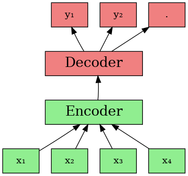
Understanding The Components

• The Input Tokens ($x_1, x_2, x_3, x_4$): In this diagram, the green boxes labeled $x_1, x_2, x_3, x_4$ represent tokens. Tokens are essentially small pieces of data—these could be whole words, subwords, or even individual characters. When you input text into an LLM, it’s broken down into these tokens. But instead of working with the raw text, the model converts these tokens into token IDs—numeric representations of each token that the model can process.

• Encoder: The encoder’s job is to take these token IDs and process them to understand the context and meaning. It creates a rich, internal representation of the input, called embeddings, that captures the relationships between the tokens.

• Decoder: After the encoder has done its work, the decoder takes over. It uses the processed information from the encoder to predict the next token in the sequence (the $y_i$s in the diagram). The decoder doesn’t just spit out a token at random, though—it uses something called a categorical distribution to make this prediction.

While there are hundreds of LLMs out there, many of them are built on variations of this encoder-decoder structure. Some models use just the encoder (like BERT), others use only the decoder (like GPT), and some use both (like T5). But no matter the variation, the basic idea remains the same: generating meaningful output tokens given a sequnce of input tokens.

How Text Generation Works

Suppose we have a vocabulary of only 10 words, including the EOS (End of Sentence) token:

Token ID	Token
0	<PAD>
1	<UNK>
2	<EOS>
3	cat
4	is
5	on
6	the
7	mat
8	dog
9	The

Now, let’s say we feed the LLM the input sentence: “The cat is on”.

The LLM processes this input and generates a categorical distribution over all possible tokens in its vocabulary. This distribution reflects the model’s prediction for what the next word should be.

Here’s what the categorical distribution might look like at this step (assuming our LLM is trained well!):

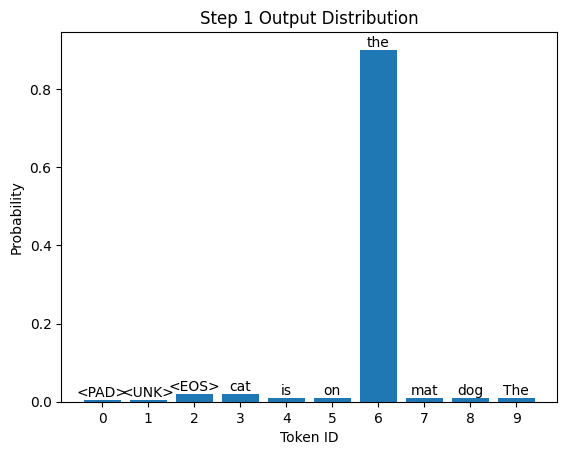
As shown in the chart, token 6 (which corresponds to "the") has the highest probability, so it’s likely to be selected as the next word. So, we have:

• Next word prediction: “the”
• Updated input: “The cat is on the”

With the updated input, the LLM generates another categorical distribution to predict the next token.

Here’s the distribution for this step:

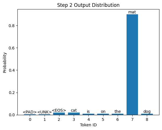
This time, token 7 (which corresponds to "mat") has the highest probability, so it’s selected as the next word.

• Next word prediction: “mat”
• Updated input: “The cat is on the mat”

The process of generating predictions continues, with the model producing distributions and selecting tokens, until it predicts the EOS token. The EOS token signals that the model should stop generating further tokens, indicating the end of the sentence.

The Challenges of Using LLMs for Time Series Forecasting

In the previous section, we saw how LLMs can generate text by predicting the next word in a sequence, using a vocabulary of discrete tokens like “cat,” “mat,” and “the.” But when it comes to time series forecasting, things get a bit more... complicated.

Challenge 1: What’s the Vocabulary of a Time Series?

In NLP, the vocabulary is pretty straightforward—it's just words. But when we step into the world of time series, we’re dealing with real numbers, which can range from negative infinity to positive infinity. Imagine trying to create a vocabulary for that!

To put it simply, there’s no neat, finite list of tokens to work with here. So, how do we even begin to define a “vocabulary” for something that could literally be anything on the number line?

Challenge 2: How Do You Tokenize a Time Series?

Even if we somehow managed to bound our time series to a finite range, we’re still left with the problem of tokenization. In NLP, we can always rely on good old whitespace (for most languages) to split text into discrete words or tokens, each with a unique ID. But if we try to tokenize time series data—say, by splitting it into daily intervals—we run into a problem: there are infinite days, just as time steps can extend indefinitely.

So, how do we break down a continuous stream of real numbers into something an LLM can actually process?

The Solution

First off, while the method we’ll discuss applies broadly to LLMs, the authors chose to experiment with T5 and GPT models.

One notable feature of this approach is that, unlike in NLP, we have the freedom to decide how many tokens we want to use to represent our time series. The authors of Chronos opted for 4096 tokens, but for simplicity and visualization, we’ll work with just 10 tokens in this blog post. However, we must reserve space for special tokens like PAD (padding) and EOS (end of sequence), leaving us with only 8 tokens for the actual time series values.

The key to the solution lies in creating bins that are mapped to token IDs. Each bin covers a specific range of numbers, so given an observation at time $t$, the token ID for that time step will depend on which bin's range the value falls into.

To make this concrete, let’s decide to support time series values in the range between -15 and 15. Besides defining these boundaries, it’s crucial to track each bin's center value (you’ll see why this matters later).

Here’s how we define the bins and their boundaries:

import numpy as np

# Define the range we want to support
LOW_LIMIT, HIGH_LIMIT = -15, 15

# Number of tokens available for actual time series data
VOCAB_SIZE = 10
N_SPECIAL_TOKENS = 2  # For PAD and EOS

# Calculate the bin centers
centers = np.linspace(LOW_LIMIT, HIGH_LIMIT, VOCAB_SIZE - N_SPECIAL_TOKENS)

# Create boundaries for binning
boundaries = np.concatenate(
    (
        np.array([-1e20]),  # To capture all lower values
        (centers[1:] + centers[:-1]) / 2,  # Midpoints between centers
        np.array([1e20]),  # To capture all higher values
    )
)

This gives the following bin centers and boundaries:

The boundaries are: [-1.00e+20, -13, -9, -4, 0, 4, 9, 13, 1.00e+20]
The centers are [-15.         -10.71428571  -6.42857143  -2.14285714   2.14285714
   6.42857143  10.71428571  15.        ]

Or, visually:

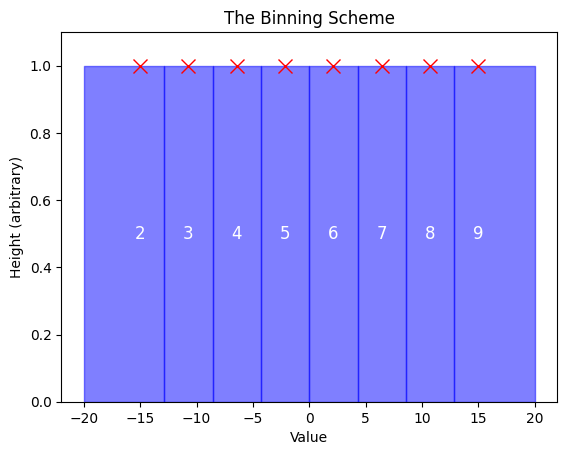
Here’s how to read the chart above:

• Eight Bins (Effective Vocabulary Size): You’ll notice that there are eight bars in the chart, corresponding to the eight available tokens we have for representing time series values. This matches our effective vocabulary size after reserving token IDs 0 and 1 for the special PAD and EOS tokens.

• Token IDs on Each Bar: The number on each bar represents the token ID assigned to that bin. We start at token ID 2 because, as mentioned, token IDs 0 and 1 are reserved for special purposes.

• Red X’s (Bin Centers): The red X’s mark the center of each bin.

• Boundaries Between Bins: The vertical lines indicate the boundaries between bins.

• First and Last Bin Boundaries: In case it's not obvious from the visual, the boundaries for the first and last bins actually start from minus infinity and end at positive infinity, respectively. This means that this binning schema will cover any value a time series can take, ensuring that no matter how extreme the values get, they’ll always be assigned to a bin.

Tokenizing Time Series Data

Now that we’ve got our binning scheme in place, the next step is to actually tokenize a time series. Let’s start with a dummy time series that we need to make a forecast from:

context = np.array([-10, 5, 100]) 

Just like an LLM can solve (or at least attempt to solve) any NLP task, we want our LLM-powered forecaster to be a universal forecaster—one that can handle any time series you throw at it. But here’s the catch: different time series can operate on vastly different scales.

For example, consider global population growth. The world’s population is measured in billions, with changes often occurring on the scale of millions or tens of millions over short periods. Contrast this with daily temperature fluctuations, which are typically measured in degrees Celsius or Fahrenheit, and often change by just a few degrees from day to day. These are two completely different scales—one operates in the billions, and the other in the single digits or tens.

To solve this, we scale the time series data using this simple function:

def mean_scale(context):
    attention_mask = ~np.isnan(context)  # Identify valid (non-NaN) values
    scale = np.nansum(np.abs(context) * attention_mask) / np.nansum(attention_mask)
    scale = max(scale, 1.0)  # Avoid division by zero or very small scales
    scaled_context = context / scale
    return scaled_context, scale, attention_mask

scaled_context, scale, attention_mask = mean_scale(context)

This function transforms the time series so that its values are typically between -1 and 1, unless the series is extremely volatile. For our example context, this gives:

Scaled Context: [-0.26086957  0.13043478  2.60869565]

We also record the input's scale—essentially the absolute mean—which will help us during the detokenization process later on:

Scale: 38.333333333333336

As for the attention mask, it’s just a mechanism to ensure that the LLM doesn’t use missing values to make predictions, and it’s not important for the purposes of this blog.

Next, we take this scaled context and assign each value to its corresponding bin, converting it into token IDs:

def tokenize(scaled_context, attention_mask):
    token_ids = np.digitize(scaled_context, bins=boundaries, right=True) + N_SPECIAL_TOKENS - 1  # -1 because np.digitize starts from 1
    token_ids[~attention_mask] = PAD_TOKEN_ID  # Mark NaNs as PAD
    return token_ids

token_ids = tokenize(scaled_context, attention_mask)
print(f"Token IDs: {token_ids}")

Which gives the following token IDs:

Token IDs: [5 6 6]

And there you have it! We’ve successfully converted a sequence of time series observations into a sequence of token IDs—the very same type of tokens that LLMs use as input. This means we can easily leverage any advances in LLMs for NLP, such as new architectures, longer context windows, or better training schemes, and apply them directly to time series forecasting. How cool is that?

Detokenizing The Model’s Output

Alright, let's do a quick recap. We’ve taken our time series, tokenized it into token IDs, and fed those into the LLM. The LLM, in turn, outputs token IDs as its prediction. But what do we do with those token IDs?

This is where the bin centers and the input's scale come into play!

Here’s the code to detokenize the predicted token IDs back into meaningful time series values:

def detokenize(token_ids, scale):
    indices = np.clip(token_ids - N_SPECIAL_TOKENS, 0, len(centers) - 1)
    scaled_values = centers[indices] * scale
    return scaled_values

For each token ID, we find the corresponding bin center, scale it back up by multiplying it with the scale we calculated earlier, when we scaled the input time series.

So, let's say we want to forecast 3 time steps ahead, and the LLM generates the following token IDs:

[3, 5, 7]

Then, the detokenized values would be:

predicted_token_ids = np.array([3, 5, 7])
predicted_values = detokenize(predicted_token_ids, scale)
print(f"Predicted Values: {predicted_values}")

Which gives:

Predicted Values: [-410.71428571  -82.14285714  246.42857143]

Sampling for Uncertainty Estimation

One of the great things about this approach is that because the forecast was generated following a sampling process, you can repeat the generation process multiple times. Each run will likely produce slightly different results, giving you a distribution of predictions. This distribution gives you a sense of the model’s confidence in its predictions.

To evaluate these predictions, you can use a metric like weighted quantile loss—which I’ve written about in an earlier post. This metric assesses the model's performance by penalizing it for wrong predictions based its confidence level.

Performance

Now that we’ve walked through how to repurpose LLMs for time series forecasting, you’re probably wondering: how well does this approach actually work?

Chronos models demonstrated exceptional performance across 42 datasets. In the in-domain Benchmark I, they outperformed classical statistical models, task-specific deep learning models, and other pretrained models , with the smallest Chronos-T5 model (Mini, 20M parameters) even surpassing much larger competitors like Moirai-1.0-R (311M parameters). In the more challenging zero-shot Benchmark II, Chronos models comfortably outperformed statistical baselines and performed on par with the best deep learning models , while also beating other leading pretrained models e.g GPT4TS. For a deeper dive into these impressive results, I highly encourage you to check out the full paper.

Conclusion

Chronos shows how innovation in LLMs can extend far beyond NLP, opening up new possibilities in time series forecasting. By adapting the techniques that have revolutionized NLP, we now have a powerful new tool to tackle time series forecasting.

I hope this blog has given you a clear understanding of how to repurpose LLMs for time series forecasting. If you have any questions or thoughts, I’d love to hear from you—drop them in the comments below, and let’s keep the conversation going!