How to do RAG without Vector Databases

Introduction

When it comes to bestowing Large Language Models (LLMs) with long-term memory, the prevalent approach often involves a Retrieval Augmented Generation (RAG) solution, with vector databases acting as the storage mechanism for the long-term memory. This begs the question: Can we achieve the same results without vector databases?

Enter "RecallM: An Adaptable Memory Mechanism with Temporal Understanding for Large Language Models" by Brandon Kynoch, Hugo Latapie, and Dwane van der Sluis. This paper proposes the use of an automatically constructed knowledge graph as the backbone of long-term memory for LLMs.

This blog post aims to delve into the mechanics of RecallM, focusing on how it updates its knowledge graph and performs inference, underpinned by a series of illustrative examples.

We'll start by exploring how the knowledge graph updates work, walking through two specific examples to clarify the process. Following that, we'll examine the inference mechanism of RecallM with another example, showcasing how it draws on the knowledge graph to generate responses. Our discussion will also cover examples of temporal reasoning, demonstrating RecallM's proficiency in understanding and applying time-based knowledge. Lastly, we'll touch upon the limitations of this approach, providing a balanced view of its capabilities and areas for further development.

Knowledge Graph Update

Round 1: Adding A New Fact

Let's say we want to add the following sentence to the knowledge graph:

Brandon loves coffee

Here's what we need to do:

Step 1: Identify the Concepts

A concept is basically a Noun in a sentence that can have a relationship with another concept.

Concepts will be nodes in the knowledge graph.

Furthermore, to avoid duplicates, we lower case and stem the concepts to their root form.

All of these can be done using an NLP package like Stanza.

Here's the annotation for the sentence "Brandon loves coffee" using Stanza:

[
  [
    {
      "id": 1,
      "text": "Brandon",
      "lemma": "Brandon",
      "upos": "PROPN",
      "xpos": "NNP",
      "feats": "Number=Sing",
      "head": 2,
      "deprel": "nsubj",
      "start_char": 0,
      "end_char": 7,
      "ner": "S-PERSON",
      "multi_ner": [
        "S-PERSON"
      ]
    },
    {
      "id": 2,
      "text": "loves",
      "lemma": "love",
      "upos": "VERB",
      "xpos": "VBZ",
      "feats": "Mood=Ind|Number=Sing|Person=3|Tense=Pres|VerbForm=Fin",
      "head": 0,
      "deprel": "root",
      "start_char": 8,
      "end_char": 13,
      "ner": "O",
      "multi_ner": [
        "O"
      ]
    },
    {
      "id": 3,
      "text": "coffee",
      "lemma": "coffee",
      "upos": "NOUN",
      "xpos": "NN",
      "feats": "Number=Sing",
      "head": 2,
      "deprel": "obj",
      "start_char": 14,
      "end_char": 20,
      "ner": "O",
      "multi_ner": [
        "O"
      ],
      "misc": "SpaceAfter=No"
    }
  ]
]

In this case, the nouns are "Brandon" and "coffee".

Stemming them using the Porter stemmer and lower casing the result, we get "brandon" and "coffe".

Step 2: Find Each Concept's Neighbors

The neighbors of a concept are the other concepts that it has a relationship with. We could use a dependency parser to find the relationships between the concepts. However, for simpplicity, we can just use the "distance" between the concepts in the sentence to determine their relationships.

"Distance" is just the position of the concept in the list of concepts extracted from the sentence. So, "brandon" is at position 0 and "coffe" is at position 0 and "coffe" is at position 1.

This code snippet will help clarify the concept of "distance":

def fetch_neigbouring_concepts(concepts, distance):
    concepts = sorted(concepts)
    for i in range(len(concepts)):
        concepts[i].related_concepts = []
        for j in range(-distance, distance + 1, 1): # If distance from current concept is less than parameter distance
            if i + j >= 0 and i + j < len(concepts): # If index is in bounds
                
                if j == 0:
                    continue

                if concepts[i].name < concepts[i+j].name: # Ensure that we only create one connection between nodes in Neo4J graph
                    concepts[i].related_concepts.append(concepts[i+j])

note

distance is set to 1 by default

The result of this step is that "brandon" has a relationship with "coffe" but "coffe" does not have a relationship with "brandon".

Step 3: Create the Concept Nodes and Relationships

We can use a graph database store the concepts and their relationships.

Here's what our knowledge graph would look like in Neo4J at the end of this step:

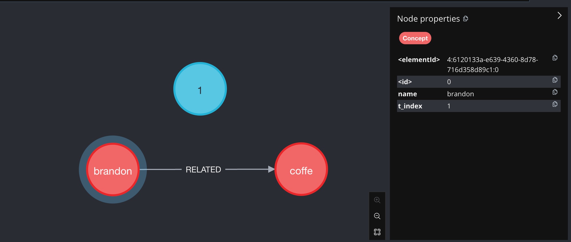Figure 1: The knowledge graph at t=1

The red nodes are the concepts. They are connected by a relationship called "RELATED" (white arrow).

The blue node is the "global timestep", which will play an important role in temporal reasoning later on. Its value is 1 because this is the first time we are updating the knowledge graph.

Here's the Cypher query to create the graph:

MERGE (c00:Concept {name: 'brandon'})
MERGE (c01:Concept {name: 'coffe'})
WITH c00, c01
MERGE (c00)-[rc00c01:RELATED]->(c01)
WITH c00, c01, rc00c01, COALESCE(rc00c01.strength, 0) + 1 AS rc00c01ic
SET c00.t_index = 1, c01.t_index = 1
SET rc00c01.strength = rc00c01ic
SET rc00c01.t_index = 1

There are 2 things to note in the Cypher query:

1. The nodes and relations have a property called t_index which is used to track when they were last updated
2. The "RELATED" relation has a property called strength which is used to track how many times the Concept it is connected to has been mentioned in the corpus used to update the knowledge graph.

Step 4: Add the Concept's Context

The context of a concept is the sentence in which it was mentioned.

So, for each concept, we first get their context from the knowledge graph:

MATCH (n:Concept)
WHERE n.name IN ['brandon', 'coffe']
RETURN n.name, n.context, n.revision_count

Of course, since this is the first time we are adding the concepts to the knowledge graph, the result of the query will be empty.

Then, we add the current context i.e. the sentence "Brandon loves coffee" to the concepts and update our knowledge graph accordingly:

MATCH (n:Concept)
WHERE n.name IN ['brandon', 'coffe']
WITH n,
        CASE n.name
                WHEN 'brandon' THEN '. Brandon loves coffee'
                WHEN 'coffe' THEN '. Brandon loves coffee'
                ELSE n.context
        END AS newContext,
        CASE n.name
                WHEN 'brandon' THEN 0
                WHEN 'coffe' THEN 0
                ELSE 0
        END AS revisionCount
SET n.context = newContext
SET n.revision_count = revisionCount

Notice that both "brandon" and "coffe" have the same context. This is because they are both mentioned in the same sentence and we have only processed one sentence so far.

This is what our knowledge graph looks like at the end of this step:

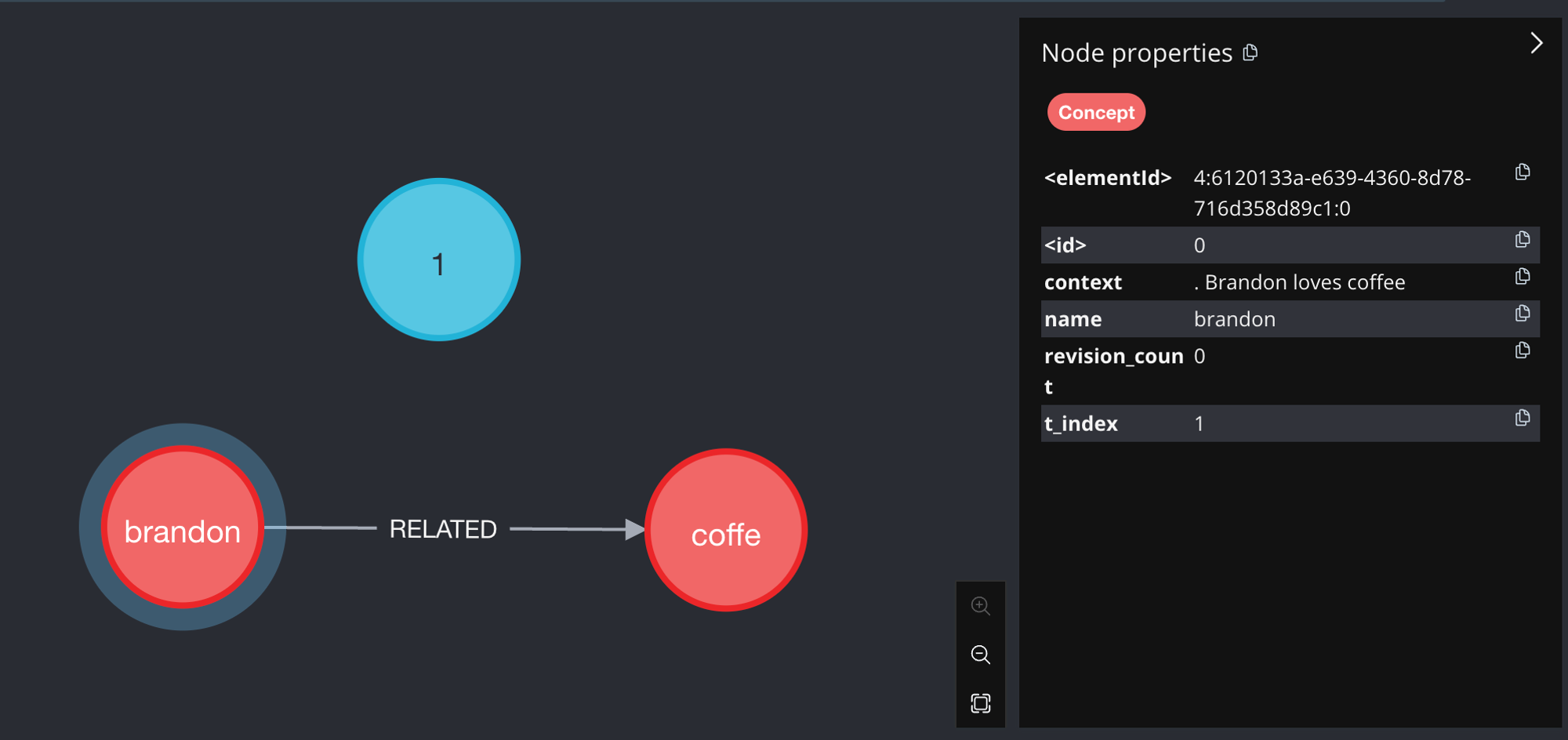Figure 2: The knowledge graph at t=1 and after adding the concept's context

note

Since a Concept node's context is regularly updated, it is possible that the concept's context will get too long too fit in an LLM's context window. This is why it is important to have another workflow that will periodically or when a concept's revision count excceds a certain threshold, summarise the context of the concepts in the knowledge graph so that it stays within the LLM's context window.

Round 2: Extending The Fact With A Another Fact

Now, let's say we want to add the following sentence to the knowledge graph:

Brandon wants to travel to Paris

You can see that the concepts in this sentence are "Brandon" and "Paris".

Stemming and lower casing them, we get "brandon" and "pari".

Adding these concepts into the knowledge graph we get:

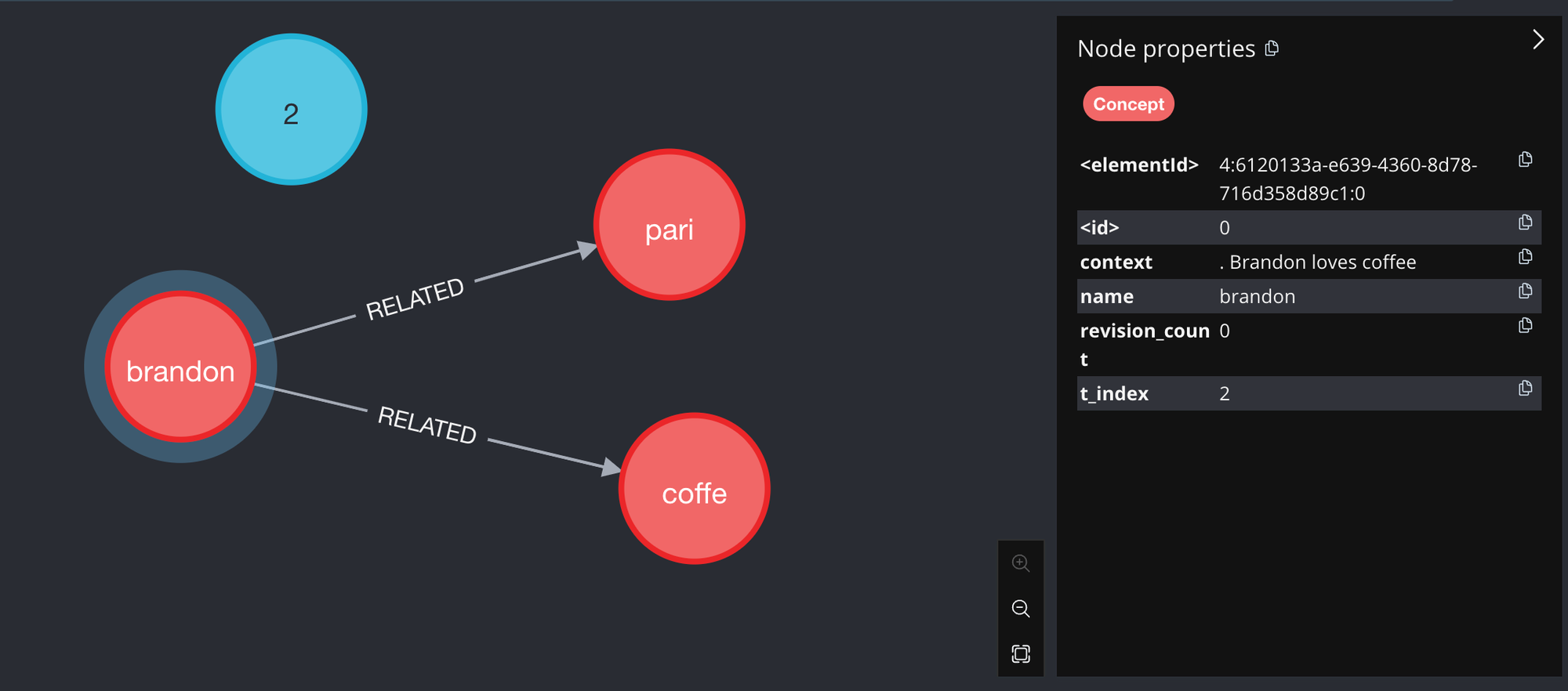Figure 3: The knowledge graph at t=2 and after adding the concepts "brandon" and "pari"

Notice that the global timestep has been updated to 2 and a new concept, "pari", has been added to the knowledge graph. "brandon" and "pari" are connected by a "RELATED" relationship. "brandon"'s t_index has been updated to 2 since it has been updated at timestep 2.

In case you are curious, here's the Cypher query to add the concepts and their relationships to the knowledge graph:

MERGE (c00:Concept {name: 'brandon'})
MERGE (c01:Concept {name: 'pari'})
WITH c00, c01
MERGE (c00)-[rc00c01:RELATED]->(c01)
WITH c00, c01, rc00c01, COALESCE(rc00c01.strength, 0) + 1 AS rc00c01ic
SET c00.t_index = 2, c01.t_index = 2
SET rc00c01.strength = rc00c01ic
SET rc00c01.t_index = 2

But what about the context of the Concept nodes?

As before, we pull the each concept's context from the knowledge graph. This time, we get the following:

{
    "brandon": {
        "context": ". Brandon loves coffee",
        "revision_count": 0
    },
    "pari": {
        "context": null,
        "revision_count": null
    }
}

As expected, "brandon" has a context while "pari" does not.

We then append the current context to the context retrieved from the knowledge graph:

MATCH (n:Concept)
WHERE n.name IN ['brandon', 'pari']
WITH n,
        CASE n.name
                WHEN 'brandon' THEN '. Brandon loves coffee. Brandon wants to travel to Paris'
                WHEN 'pari' THEN '. Brandon wants to travel to Paris'
                ELSE n.context
        END AS newContext,
        CASE n.name
                WHEN 'brandon' THEN 1
                WHEN 'pari' THEN 0
                ELSE 0
        END AS revisionCount
SET n.context = newContext
SET n.revision_count = revisionCount

Notice that "brandon" has a new context that includes the previous context and the new sentence. Its revision_count has been updated to 1 too because it has been updated with a new context.

This is what our knowledge graph looks like at the end of this step:

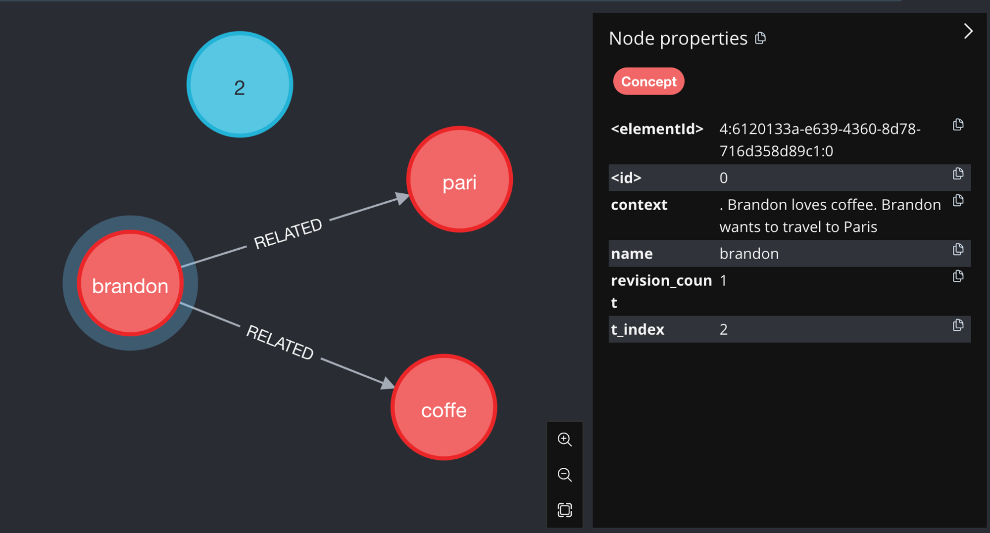Figure 4: The knowledge graph at t=2 and after adding the concept's context

Inference Mechanism

Let's say we want to generate a response to the question:

Who wants to travel to Paris?

Here's how we can use the knowledge graph to generate the response:

Step 1: Identify The Concepts

Using the same NLP pipeline we used to identify the concepts in the sentences we used to update the knowledge graph, we determine that there's only one concept in the question: "pari".

Step 2: Find The Related Concepts

We use our knowledge graph to find the concepts that are related to "pari":

MATCH (startNode:Concept{name: 'pari'})
CALL apoc.path.spanningTree(startNode, {relationshipFilter: "", minLevel: 0, maxLevel: 2}) YIELD path
WITH path, nodes(path) as pathNodes, startNode.t_index as current_t
UNWIND range(0, size(pathNodes)-1) AS index
WITH path, pathNodes[index] as node, current_t
ORDER BY node.t_index DESC
WHERE node.t_index <= current_t AND node.t_index >= current_t - 15
WITH DISTINCT node LIMIT 800
MATCH ()-[relation]->()
RETURN node, relation

The above query finds all paths up to 2 levels deep starting from the "pari" Concept node, filters the resulting nodes based on their t_index to ignore concepts younger and older than 15 timesteps relative to "pari", takes the first 800 unique nodes, and returns these nodes and relationships in the graph.

This results in the following concept nodes:

{
    "pari": ". Brandon wants to travel to Paris",
    "brandon": ". Brandon loves coffee. Brandon wants to travel to Paris",
    "coffe": ". Brandon loves coffee"
}

Step 3: Rank The Related Concepts

We rank the each of the related concepts based on their t_index and the strength of the relationship between them and their own related concepts.

For the sake of clarity, here's the code snippet that does this:

 graph_concepts = graph_concept_nodes.values()
    for concept in graph_concepts:
        concept.sort_val = 0
        for relation in concept.related_concepts:
            concept.sort_val += (relation.t_index * 3) + relation.strength     # TODO: 3 is a hyperparameter, move this to header
    graph_concepts = sorted(graph_concepts, key=lambda c: c.sort_val)
    graph_concepts.reverse()    # We want them in descending order, so that highest temporal relations are first

The "score" is called sort_val in the code snippet. The higher the sort_val, the more temporally relevant the concept is.

If you want to follow along, here's the sort_val for each concept that was found to be related to "pari":

Concept	Context	t_index	sort_val
brandon	Brandon loves coffee. Brandon wants to travel to Paris	2	11
pari	Brandon wants to travel to Paris	2	7
coffe	Brandon loves coffee	1	4

Step 4: Build The Context

We start with the context of the concept that are present in the question. We call this the "essential concepts". In this case, it's just "pari".

And the context is just the sentence "Brandon wants to travel to Paris".

Then, we prepend to that the context of the concepts found in the previous step, in order of descending sort_val.

This gives us the following context to be passed to the LLM:

. Brandon loves coffee # from related concept: coffee

. Brandon loves coffee. Brandon wants to travel to Paris # from related concept: brandon

. Brandon wants to travel to Paris # from essential concepts

Step 5: Generate The Response

All that's left is to prompt the LLM with the context we built in the previous step and let it generate the response.

The prompt would look something like this:

Using the following statements when necessary, answer the question that follows. Each sentence in the following statements is true when read in chronological order: 

statements:
. Brandon loves coffee

. Brandon loves coffee. Brandon wants to travel to Paris

. Brandon wants to travel to Paris

question:
Who wants to travel to Paris?

Answer:

With such a comprehensive and well-thought-out prompt, the LLM, using gpt-3.5-turbo in this case, is be able to generate the correct response: 'Brandon'.

Temporal Reasoning

The authors designed a simple experiment to evaluate RecallM's temporal understanding and memory updating abilities. They created a dataset consisting of chronological statements, with each subsequent statement representing the current truth over previous ones. The system was questioned at regular intervals to gauge its comprehension of temporal concepts, including the order of events and knowledge from previous statements.

The experiment included two sets of questions: standard temporal questions and long-range temporal questions. The former tested the system's understanding of temporal concepts and its ability to update beliefs and memories, while the latter required recalling information provided hundreds of statements ago. To correctly answer long-range questions after 25 repetitions, the system needed to recall and reason about knowledge from over 1,500 updates prior.

Here are some examples the paper shared about this experiment, highlighting the efficacy of the RecallM architecture in retaining and utilizing temporal knowledge:

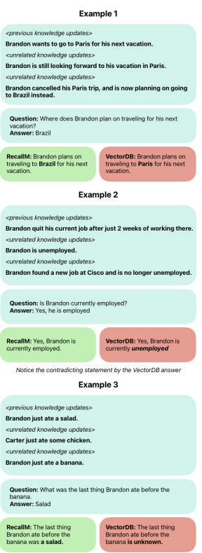
Figure 5: RecallM vs Vector DB on temporal reasoning

Limitations

The major limitation of this approach lies in the construction of the knowledge graph. In particular, it is lacking coreference resolution.

What this means is that if we feed it the following text:

Brandon loves coffee. He wants to travel to Paris. He likes cats.

We would expect the knowledge graph to look like this:

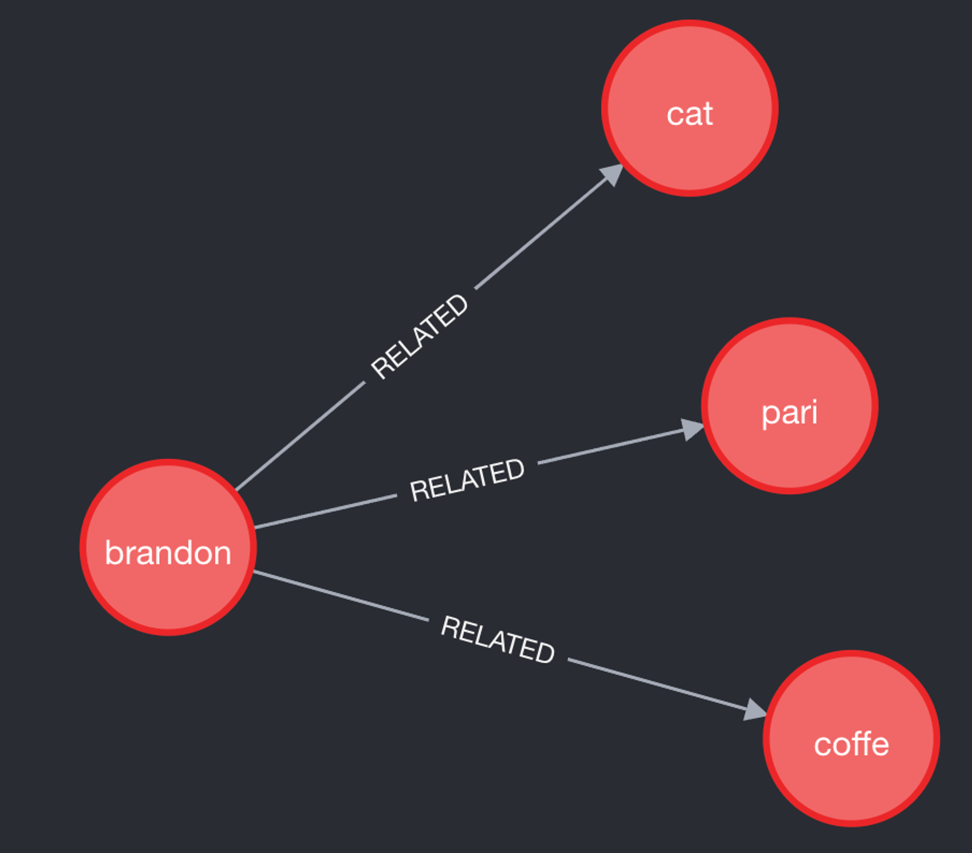Figure 6: Expected knowledge graph

However, we actually end up with this:

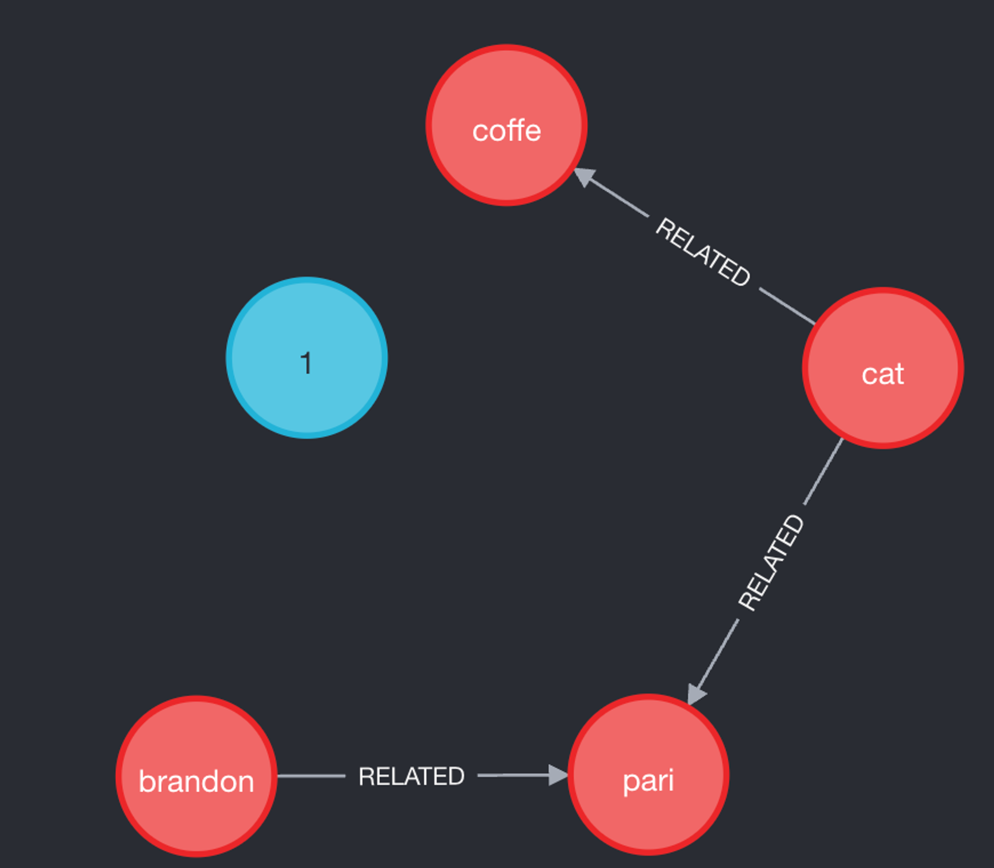Figure 7: Actual knowledge graph

Nevertheless, asking questions like:

• Who wants to travel to Paris?
• Who likes cats?
• Who loves coffee?

Would still yield the correct answer, as the resulting context would still have "Brandon loves coffee" in it which helps the LLM generate the correct response. I'm not sure if there are edge cases where this would not be the case.

A solution to this could be to translate a text passage into "propositions" as discussed in the paper "Dense X Retrieval: What Retrieval Granularity Should We Use?" by Chen et. al., and feed those propositions into the knowledge graph instead of the raw text passage.

Conclusion

In summary, RecallM presents an interesting method for integrating long-term memory into LLMs using only a graph database. While demonstrating effectiveness in updating stored knowledge and temporal understanding, challenges like creating accurate knowledge graphs persist. Nonetheless, it is a notable advancement in AI systems, with ongoing research offering opportunities for refinement and improvement.